Theory

When we talk about the “control” of a system, we broadly refer to some input or change to the system that alters its behavior in a desired way. To more precisely discuss control, we first have to discuss the object that is being controlled: the system. In the network control framework, what is being controlled is a dynamical system.

What is a Dynamical System?

As per the Wikipedia article on dynamical systems: “a dynamical system is a system in which a function describes the time dependence of a point in geometrical space.” We’re going to reword this sentence a bit to say: “a dynamical system is a system whose states evolve forward in time in geometric space according to a function.” Let’s unpack this sentence a bit.

“A dynamical system is a system”

The word “dynamic” (change) is used in contrast to “static” (no change). If a system is dynamic, it changes over time. That’s all well and good, but what exactly is changing about the system? The answer is: the states.

“whose states”

A state is just a complete description of a system. Take for example a train. If I know the position \(x\) of the train from some station, then I know exactly where the train is. It can only move forwards or backwards along the track, and every position along that track has an associated position \(x\), or state. As another example, in a computer, if I know the voltage of every single transistor, then I have a complete description of the computer, and I can unambiguously describe all possible states of the computer using these transistor voltages (states).

“evolve forward in time”

When we say dynamic (states are changing), we mean to say that the states are changing forward in time. Hence, time is a very important concept in dynamical systems. The field of dynamical systems broadly concerns itself with the question “how do the system states evolve forward in time?”

“in geometric space”

When we say “geometric,” we usually mean the colloquial usage of the word. That is, Euclidean space. We live in 3-dimensional Euclidean space, where every point is described by 3 coordinates: \((x,y,z)\). In a dynamical system, there is no need to restrict ourselves to 3 dimensions. In the train example, we can represent the position of the train along the track, \(x\), on a number line. Even if the track itself is not straight, we can “straighten out” the track to form a 1-dimensional line. As another exmple, the FitzHugh-Nagumo model is a 2-dimensional simplification of a Hodgkin-Huxley neuron, with two states, \(v\) and \(w\). We can plot these states separately over time (left,center), or we can plot them together in a 2-dimensional geometric space, where each axis represents either \(v\) or \(w\) (right).

“according to a function.”

Now, just because a system has states and evolves forward in time does not make it a dynamical system. For a system to be dynamical, it must evolve forward in time according to a function. This requirement is precisely where differential equations enters the fray. Specifically, the function that the dynamical system uses to evolve forward in time is a differential equation. For example, the FitzHugh-Nagumo model evolves according to the functions

\[\begin{split}\frac{\mathrm{d}v}{\mathrm{d}t} &= v - \frac{v^3}{3} - w + 0.5\\ \frac{\mathrm{d}w}{\mathrm{d}t} &= \frac{1}{12.5} (v + 0.8 - 0.7w)\\\end{split}\]

What is a Differential Equation?

As per the Wikipedia definition: “a differential equation is an equation that relates one or more functions and their derivatives.” Let’s break down this sentence.

“A differential equation is an equation”

An equation is a relation that equates the items left of the equal sign to the items right of the equal sign. For example, for a right triangle with side lengths \(a,b\) and hypotenuse length \(c\), the Pythagorean equation is:

\[c^2 = a^2 + b^2\]

This equation has thre evariables that are related by one equation. Hence, if I fix \(a\) and \(b,\) then I know what \(c\) has to be for the triangle to be a right triangle.

“that relates one or more functions and their derivatives.”

A derivative is an operation that tells us how a variable changes. For example, if \(c\) is a variable measuring the side length of the triangle, then \(\mathrm{d}c\) is a variable measuring the change in that side length. Typically, these change variables come as ratios to measure how quickly one variable changes with respect to another variable. For example, \(\frac{\mathrm{d}c}{\mathrm{d}a}\) is a ratio between a change in \(c\) with respect to a change in \(a\).

Dynamical Systems & Differential Equations

Recall the two statements that we have made thus far:

• Dynamical system: a system whose states evolve forward in time in geometric space according to a function

• Differential equation: an equation that relates one or more functions and their derivatives.

Hence the relationship between these two is that the function is a differential equation of derivatives. In particular, the derivative of the system states with respect to time.

In the differential equations of a dynamical system, the left-hand side contains a derivative of the state with respect to time, \(\frac{\mathrm{d}x}{\mathrm{d}t}.\) The right-hand side contains a function of the states, \(f(x).\) Hence, generally speaking, a dynamical equation looks like

\[\frac{\mathrm{d}x}{\mathrm{d}t} = f(x).\]

As a specific example, let’s look at the dynamical equation

\[\frac{\mathrm{d}x}{\mathrm{d}t} = -x,\]

and let’s see what happens at some specific states.

• If \(x=1,\) then \(\frac{\mathrm{d}x}{\mathrm{d}t} = -1.\) In other words, if the system state is at 1, then the change in state with respect to time is negative, such that the state moves towards 0.

• If \(x=-1,\) then \(\frac{\mathrm{d}x}{\mathrm{d}t} = 1.\) In other words, if the system state is at -1, then the change in state with respect to time is positive, such that the state moves towards 0.

• If \(x=0,\) then \(\frac{\mathrm{d}x}{\mathrm{d}t} = 0.\) The system does not change, and the state remains at 0.

If we plot the trajectories \(x(t)\) over time (left), we see that, as predicted, the trajectories all move towards \(0\) (left), and that the change in the state, \(\frac{\mathrm{d}x}{\mathrm{d}t},\) also points towards \(0\) (right).

Hence, the dynamical equation for a system describes the evolution of the state at every point in state space. To visualize this description in 2-dimensions, let us revisit the equations for the FitzHugh-Nagumo model,

\[\begin{split}\frac{\mathrm{d}v}{\mathrm{d}t} &= v - \frac{v^3}{3} - w + 0.5\\ \frac{\mathrm{d}w}{\mathrm{d}t} &= \frac{1}{12.5} (v + 0.8 - 0.7w),\end{split}\]

and at every point \((v,w)\), we will draw an arrow pointing towards \((\mathrm{d}v/\mathrm{d}t, \mathrm{d}w/\mathrm{d}t).\)

We observe that at every point in the state space, we can draw an arrow defined by the dynamical equations. Additionally, we observe that the evolution of the system states, \(v(t)\) and \(w(t),\) follow these arrows. Hence, the differential equations define the flow of the system states over time.

For convenience, we will name all of our state varibles \(x_1,x_2,\dotsm,x_N,\) and collect them into an \(N\)-dimensional vector \(\mathbf{x}.\) For an additional convenience, instead of always writing the fraction \(\frac{\mathrm{d}x}{\mathrm{d}t},\) we will use \(\dot{x}\) to represent the time derivative of \(x.\)

Linear State-Space Systems

Now that we have a better idea of what a dynamical system is, we would like to move on to control. However, there is a fundamental limitation when attempting to control a system, which is that we do not know how the system will naturally evolve. At any given state, \(\mathbf{x}(t),\) we can use the dynamical equations to know where the state will immediately go, \(\frac{\mathrm{d}\mathbf{x}(t)}{\mathrm{d}t}.\) However, we generally cannot know where the state will end up after a finite amount of time, at \(\mathbf{x}(t+T).\) This problem extends to any perturbation we perform on the system, where we cannot know how the perturbation will affect the state after a finite amount of time.

However, there is a class of dynamical systems where we can know both where the states will end up, and how a perturbation will change the states after a finite amount of time. These systems are called linear time-invariant systems, or LTI systems.

scalar LTI system

We have already looked at an example of an LTI system, namely,

\[\frac{\mathrm{d}x}{\mathrm{d}t} = -x.\]

We can make this system a bit more general, and look at

\[\frac{\mathrm{d}x}{\mathrm{d}t} = ax,\]

where \(a\) is a constant real number. Using some basic calculus, we can actually solve for the trajectory \(x(t).\) First, we divide both sides by \(x\) and multiply both sides by \(a\) to match terms,

\[\frac{1}{x}\mathrm{d}x = a\mathrm{d}t.\]

Then, we integrate both sides,

\[\begin{split}\int \frac{1}{x} \mathrm{d}x &= \int a \mathrm{d}t + c\\ \ln|x| &= at + c.\end{split}\]

Finally, we exponentiate both sides to pull out \(x(t)\):

\[x(t) = Ce^{at},\]

where the constant \(C\) is the initial condition, \(C = x(0).\) This is because when we plug in \(t=0,\) the exponential becomes \(e^{a0} = 1.\) Hence, we can write our final trajectory as

\[x(t) = x(0) e^{at},\]

which tells us exactly what the state of our system will be at every point in time. This knowledge of the state at every point in time is generally very difficult to obtain for nonlinear systems. To verify that this trajectory really is a solution to our dynamical equation, we can substitute it back into the differential equation, and check if the left-hand side equals the right-hand side. To evaluate the left-hand side, we must take the time derivative of \(e^{at},\) which we can do by writing the exponential as a Taylor series, such that \(e^{at} = \sum_{k=0}^\infty \frac{(at)^k}{k!}.\) Then taking the derivative of each term with respect to time, we get

\[\begin{split}\frac{\mathrm{d}}{\mathrm{d}t}e^{at} &= \frac{\mathrm{d}}{\mathrm{d}t} \left( 1 + \frac{at}{1!} + \frac{a^2t^2}{2!} + \frac{a^3t^3}{3!} + \dotsm + \frac{a^kt^k}{k!} + \dotsm\right)\\ &= 0 + \frac{a}{1!} + 2\frac{a^2t}{2!} + 3\frac{a^3t^2}{3!} + \dotsm + k\frac{a^lt^{k-1}}{k!} + \dotsm\\ &= a\left(1 + \frac{at}{1!} + \frac{a^2t^2}{2!} + \dotsm + \frac{a^kt^k}{k!}\right)\\ &= ae^{at}.\end{split}\]

Hence, the derivative of \(e^{at}\) is equal to \(ae^{at},\) such that the left-hand side of the dynamical equation equals the right-hand side.

vector LTI system

Of course, systems like the brain typically have many states, and writing down the equations for all of those states would be quite tedious. Fortunately, we can obtain all of the results in scalar LTI systems for vector LTI systems using matrix notation. In matrix form, the state-space LTI dynamics are written as

\[\begin{split}\underbrace{\begin{bmatrix} \dot{x}_1\\\dot{x}_2\\\vdots\\\dot{x}_N \end{bmatrix}}_{\dot{\mathbf{x}}} = \underbrace{\begin{bmatrix} a_{11} & a_{12} & \dotsm & a_{1N}\\ a_{21} & a_{22} & \dotsm & a_{2N}\\ \vdots & \vdots & \ddots & \vdots\\ a_{N1} & a_{N2} & \dotsm & a_{NN} \end{bmatrix}}_{A} \underbrace{\begin{bmatrix} \dot{x}_1\\\dot{x}_2\\\vdots\\\dot{x}_N \end{bmatrix}}_{\mathbf{x}},\end{split}\]

or, more compactly, as

\[\dot{\mathbf{x}} = A\mathbf{x}.\]

Here, \(a_{ij}\) is the element in the \(i\)-th row and \(j\)-th column of matrix \(A,\) and represents the coupling from state \(j\) to state \(i.\)

Now, it might be too much to hope that the solution to the vector LTI system is simply a matrix version of the scalar form, perhaps something like \(\mathbf{x}(t) = e^{At}\mathbf{x}(0).\) However, this form is precisely the solution to the vector dynamical equation! Exactly as in the scalar version, we can write the matrix exponential, \(e^{At},\) as a Taylor series such that \(e^{At} = \sum_{k=0}^\infty \frac{(At)^k}{k!},\) and again take the time derivative of each term to get

\[\begin{split}\frac{\mathrm{d}}{\mathrm{d}t}e^{At} &= \frac{\mathrm{d}}{\mathrm{d}t} \left( 1 + \frac{At}{1!} + \frac{A^2t^2}{2!} + \frac{A^3t^3}{3!} + \dotsm + \frac{A^kt^k}{k!} + \dotsm\right)\\ &= 0 + \frac{A}{1!} + 2\frac{A^2t}{2!} + 3\frac{A^3t^2}{3!} + \dotsm + k\frac{A^lt^{k-1}}{k!} + \dotsm\\ &= A\left(1 + \frac{At}{1!} + \frac{A^2t^2}{2!} + \dotsm + \frac{A^kt^k}{k!}\right)\\ &= Ae^{at}.\end{split}\]

Hence, the trajectory of a vector LTI system is given simply by

\[\mathbf{x}(t) = e^{At}\mathbf{x}(0).\]

In general, \(e^{At}\) is called the impulse response of the system, because for any impulse \(\mathbf{x}(0),\) the impulse response tells us precisely how the system will evolve.

The Potential of Linear Response

Until now, we have written down several examples of systems that we have called linear. Drawing on our prior coursework in linear algebra, we recall that the adjective linear is used to describe a particular property of some operator \(f(\cdot)\) acting on some objects \(x_1,x_2.\) That is, if

\[y_1 = f(x_1) ~\mathrm{and}~ y_2 = f(x_2),\]

then \(f(\cdot)\) is linear if

\[a y_1 + b y_2 = f(a x_1 + b x_2 ).\]

Colloquially, if an operator is linear, then it adds distributively. Scaling the input by a constant scales the output by the same constant, and the sum of two inputs yields the sum of the outputs.

So then, what do we mean when we say that our dynamical system is linear? In this case, we mean that the impulse response is linear. That is, for two initial conditions, \(\mathbf{x}_1(0), \mathbf{x}_2(0),\) if

\[\mathbf{x}_1(t) = e^{At}\mathbf{x}_1(0) ~\mathrm{and}~ \mathbf{x}_2(t) = e^{At}\mathbf{x}_2(0),\]

then

\[a \mathbf{x}_1(t) + b \mathbf{x}_2(t) = e^{At}(a\mathbf{x}_1(0) + b\mathbf{x}_2(0)),\]

which is true by the distributive property.

a 2-state example

While this property might not seem so impressive at first glance, the implications are actually quite powerful. Specifically, this linearity allows us to write all possible trajectories of our system as a simple weighted sum of initial conditions. Hence, rather than having to simulate all initial states to see if we reach a particular final state, we can reconstruct the initial state that yields a desired final state. To demonstrate, consider the following simple 2-dimensional system

\[\begin{split}\begin{bmatrix} \dot{x}_1\\ \dot{x}_2\end{bmatrix} = \begin{bmatrix} -1 & -2\\ 1 & 0\end{bmatrix},\end{split}\]

and two initial conditions

\[\begin{split}\mathbf{x}_1(0) = \begin{bmatrix}1\\0\end{bmatrix}, \hspace{1cm} \mathbf{x}_2(0) = \begin{bmatrix}0\\1\end{bmatrix}.\end{split}\]

Evolving these two states until \(T=1\) yields final states

\[\begin{split}\mathbf{x}_1(T) = \begin{bmatrix}-0.0734\\0.4445\end{bmatrix}, \hspace{1cm} \mathbf{x}_2(T) = \begin{bmatrix}-0.8890\\0.3711\end{bmatrix},\end{split}\]

and we can plot the trajectories towards those final states below (left).

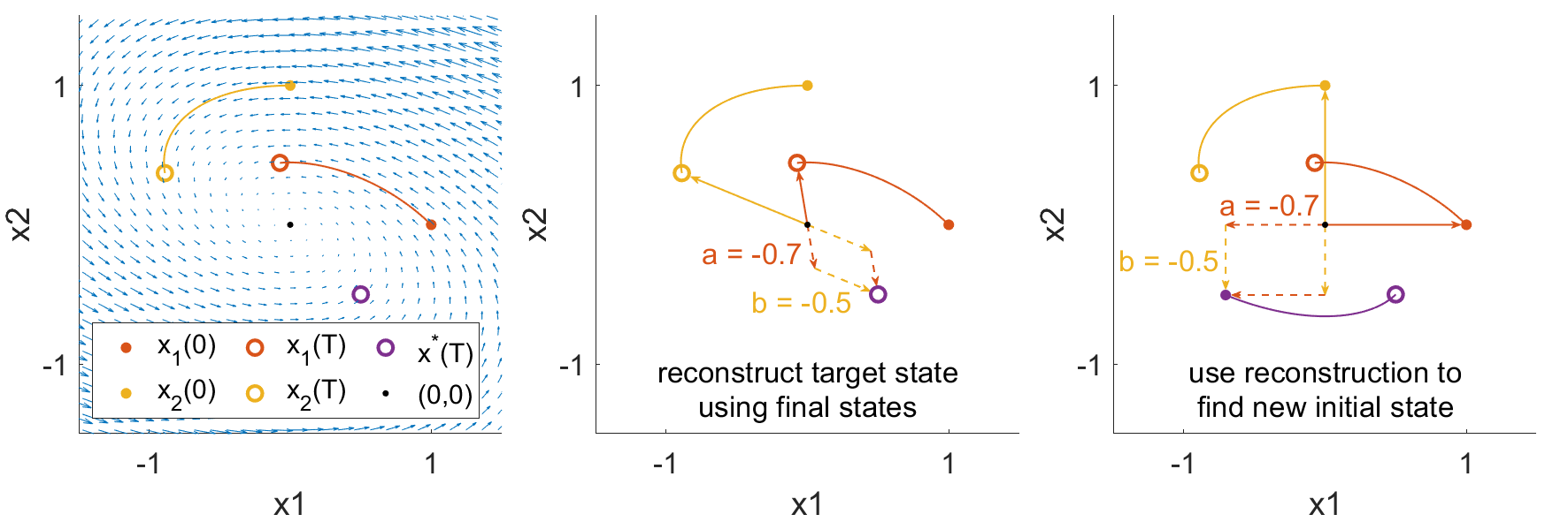
Now, suppose we wanted the system to actually reach a different final state, say

\[\begin{split}\mathbf{x}^*(T) = \begin{bmatrix}0.5\\-0.5\end{bmatrix}.\end{split}\]

Because of the linearity of the system, we know that weighted sums of the initial states map to the same weighted sums of the trajectories. We can reverse this idea and write the desired final state as a weighted sum of trajectories,

\[\begin{split}\mathbf{x}^*(T) = a\mathbf{x}_1(T) + b\mathbf{x}_2(T) = \begin{bmatrix} \mathbf{x}_1(T) & \mathbf{x}_2(T)\end{bmatrix} \begin{bmatrix} a\\b \end{bmatrix},\end{split}\]

and solve for the weights through simple matrix inversion

\[\begin{split}\begin{bmatrix} a\\b \end{bmatrix} = \begin{bmatrix} \mathbf{x}_1(T) & \mathbf{x}_2(T)\end{bmatrix}^{-1} \mathbf{x}^*(T) = \begin{bmatrix}-0.7\\-0.5\end{bmatrix}.\end{split}\]

Then, if we use the same weighted sums of the initial states, then the new initial state is guaranteed to reach the desired target state,

\[\mathbf{x}^*(0) = a\mathbf{x}_1(0) + b\mathbf{x}_2(0),\]

due to the properties of linearity such that

\[\begin{split}e^{AT}\mathbf{x}^*(0) &= e^{AT}(a\mathbf{x}_1(0) + b\mathbf{x}_2(0))\\ ~&= ae^{AT}\mathbf{x}_1(0) + be^{AT}\mathbf{x}_2(0)\\ ~&= a\mathbf{x}_1(T) + b\mathbf{x}_2(T)\\ ~&= \mathbf{x}^*(T).\end{split}\]

As we can see, we did not have to do any guesswork in solving for the initial state that yielded the desired final state. Instead, we reconstructed the final state from a basis of final states, and took advantage of the linear property of the impulse response to apply that reconstruction to the initial states. This reconstruction using basis vectors and linearity is the core principle behind network control theory.

an easier approach

While the previous reconstruction example was useful, the linearity of the impulse response actually allows us to solve the problem much faster, because at the end of the day, the impulse response is simply a linear system of equations,

\[\mathbf{x}(T) = e^{AT}\mathbf{x}(0).\]

So, we know \(A,\) and we know the desired target state, \(\mathbf{x}(T),\) so we just multiply both sides of the equation by the inverse of \(e^{AT}\) to yield the correct initial state

\[\begin{split}\mathbf{x}(0) = e^{-AT} \mathbf{x}(T) = \begin{bmatrix} -0.7\\ -0.5 \end{bmatrix}.\end{split}\]

And… that’s kind of it. And fundamentally, the control of these systems uses the exact same idea. That is, we find some linear operation that takes us from the control input to the final state, then solve for the input using some fancy versions of matrix inverses.

Controlled Dynamics

Until now, we have worked with LTI dynamics, which we write as

\[\dot{\mathbf{x}} = A\mathbf{x}.\]

When we say control, we intend to perturb the system using some external inputs, \(u_1(t), u_2(t),\dotsm,u_k(t),\) that we will collect into a vector \(\mathbf{u}(t).\) These inputs might be electromagnetic stimulation from transcranial magnetic stimulation (TMS), some modulation of neurotransmitters through medication, or sensory inputs. And of course, these inputs don’t randomly affect all brain states separately, but have a specific pattern of effect based on the site of stimulation, neurotransmitter distribution, or sensory neural pathways. We represent this mapping from stimuli to brain regions through vectors \(\mathbf{b}_1,\mathbf{b}_2,\dotsm,\mathbf{b}_k,\) which we collect into an \(N\times k\) matrix \(B.\) Then our new controlled dynamics become

\[\dot{\mathbf{x}} = A\mathbf{x} + B\mathbf{u}.\]

So now we have a bit of a problem. We would like to write \(\mathbf{x}(t)\) as some nice linear function as before, but how do we do this? The derivation requires a bit of algebra, so feel free to skip it!

derivation of the controlled response

So the first thing we will try to do is, as before, move all of the same variables to one side. So first, we will subtract both sides by \(A\mathbf{x}\)

\[\dot{\mathbf{x}} - A\mathbf{x} = B\mathbf{u}.\]

Then, as before, we want to integrate the time derivative. However, simply integrating both sides will yield a \(\int A\mathbf{x}\) term, which we do not want. To combine the \(\dot{\mathbf{x}}\) and \(A\mathbf{x}\) terms, we will first mutiply the equation by :math:e^{-At},

\[e^{At}\dot{\mathbf{x}} - e^{At}A\mathbf{x} = e^{At}B\mathbf{u},\]

and notice that we can actually perform the reverse of the product rule on the left-hand side. Specifically, \(\frac{\mathrm{d}}{\mathrm{d}t} e^{At}\mathbf{x} = e^{At}\dot{\mathbf{x}} - e^{At}A\mathbf{x}\) (small note, \(e^{-At}A = Ae^{-At}\) because a matrix and functions of that matrix commute). Substituting this expression into the left-hand side, we get

\[\frac{\mathrm{d}}{\mathrm{d}t} e^{At}\mathbf{x} = e^{At}B\mathbf{u}\]

Now we are almost done, as we integrate both sides from \(t = 0\) to \(t = T\) to yield

\[e^{-AT} \mathbf{x}(T) - \mathbf{x}(0) = \int_0^T e^{-At} B\mathbf{u}(t) \mathrm{d}t\]

Finally, we isolate the term \(\mathbf{x}(T)\) by adding both sides of the equation by \(\mathbf{x}(0),\) and multiplying through by \(e^{AT}\) to yield

\[\underbrace{\mathbf{x}(T)}_{\mathrm{target}} = \underbrace{e^{AT}\mathbf{x}(0)}_{\mathrm{natural}} + \underbrace{\int_0^T e^{A(T-t)} B\mathbf{u}(t) \mathrm{d}t}_{\mathrm{controlled}}\]

We notice that the first term, the “natural” term, is actually our original, uncontrolled impulse response. We also notice that the second term, the “controlled” term, is just a convolution of our input, \(\mathbf{u}(t),\) with the impulse response. For conciseness, we will write the convolution using a fancy letter \(\mathcal{L}(\mathbf{u}) = \int_0^T e^{A(T-t)} B\mathbf{u}(t) \mathrm{d}t,\) and rewrite our controlled response as

\[\underbrace{\mathbf{x}(T)}_{\mathrm{target}} = \underbrace{e^{AT}\mathbf{x}(0)}_{\mathrm{natural}} + \underbrace{\mathcal L(\mathbf{u}(t))}_{\mathrm{controlled}}\]

some intuition for the controlled response

We can gain some simple intuition by rearranging the controlled response a little

\[\underbrace{\mathbf{x}(T)}_{\mathrm{target}} - \underbrace{e^{AT}\mathbf{x}(0)}_{\mathrm{natural}} = \underbrace{\mathcal L(\mathbf{u}(t))}_{\mathrm{controlled}}\]

If we look closely, we notice that the controlled response simply makes up the difference between the natural evolution of the system from its initial state, and the desired target state. To visualize this equation in our previous 2-dimensional example, we mark the initial state and natural evolution of the initial state in orange, and the desired target state in purple. The controlled response is algebraically responsible for making up the gap between the initial and target state.

The Potential of Linear Controlled Response

So now we reach the final question: how do we design the controlled response, \(\mathbf{u}(t),\) that brings our system from an initial state \(\mathbf{x}(0)\) to a desired target state \(\mathbf{x}(T)\) ? And the great thing about this question is that we already know how to do it because the controlled response is linear. By linear, we again mean that for some input \(\mathbf{u}_1(t)\) that yields an output \(\mathbf{y}_1 = \mathcal L(\mathbf{u}_1(t)),\) and another input \(\mathbf{u}_2(t)\) that yields an output \(\mathbf{y}_2 = \mathcal L(\mathbf{u}_2(t)),\) we have that

\[a\mathbf{y}_1 + b\mathbf{y}_2 = \mathcal L(a\mathbf{u}_1 + b\mathbf{u}_2)\]

This fact comes from the fact that the convolution operator is linear.

a simple 2-state example

So let’s try to derive some intuition with the same 2-state example as before, but now our system will have a controlled input such that

\[\begin{split}\underbrace{\begin{bmatrix} \dot{x}_1\\ \dot{x}_2\end{bmatrix}}_{\dot{\mathbf{x}}} = \underbrace{\begin{bmatrix} -1 & -2\\ 1 & 0\end{bmatrix}}_{A} \underbrace{\begin{bmatrix} x_1\\ x_2\end{bmatrix}}_{\mathbf{x}} + \underbrace{\begin{bmatrix} 1 & 0\\ 0 & 1 \end{bmatrix}}_{B} \underbrace{\begin{bmatrix} u_1\\u_2 \end{bmatrix}}_{\mathbf{u}}.\end{split}\]

The natural trajectory of the system is shown as the blue curve, while the first controlled trajectory when \(u_1=1\) is shown in the red curve, and the second controlled trajectory when \(u_2=1\) is shown in the yellow curve (left).

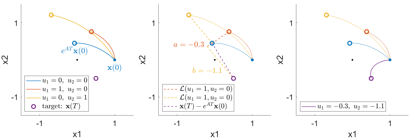
Now, we have to be careful about exactly what is linear. And the thing that is linear is the convolution operator, \(\mathcal{L}(\mathbf{u}) = \int_0^T e^{A(T-t)} B\mathbf{u}(t) \mathrm{d}t.\) This operator takes the control input, \(\mathbf{u}(t),\) as its input, and outputs the difference between the final state, \(\mathbf{x}(T),\) and the natural, uncontrolled evolution, \(e^{AT} \mathbf{x}(0).\) Hence, we have to speak about the states relative to the natural, uncontrolled evolution.

So when we look at the effect of the first controlling input \(u_1=1,\) we are looking at the difference between the controlled final state (open orange circle) from the natural final state (open blue circle). Similarly, when we look at the effect of the second controlling input \(u_2 = 1,\) we are looking at the difference between the controlled final state (open yellow circle) from the natural final state (open blue circle). And if we want to reach a new target state (open purple circle), we use these differences in controlled trajectories (dashed red and yellow lines) as the basis vectors, and find the weighted sums that yield the difference between the target state and the natural final state (dashed purple line), which yields \(u_1 = -0.3, u_2 = -1.1.\) And when we control our system using this linear combination of inputs, we see that the trajectory indeed reaches the desired target state (right).

Minimum Energy Control

Of course, this process is all a bit tedious, because we first have to simulate controlled trajectories, then take combinations of those trajectories. Is there a faster and easier way to solve for control inputs that perform a state transition without having to run simulations? The answer is yes, because the controlled response operator \(\mathcal L(\mathbf{u})\) is linear, but requires a bit of care.

So first, let’s think about a typical linear regression problem, \(M\mathbf{v} = \mathbf{b},\) where \(M\) is an \(k \times n\) matrix, \(\mathbf{v}\) is an \(n\) dimensional vector, and \(\mathbf{b}\) is an \(k\) dimensional vector,

\[\begin{split}\underbrace{\begin{bmatrix} m_{11} & m_{12} & m_{13} & \dotsm & m_{1n}\\ m_{21} & m_{22} & m_{23} & \dotsm & m_{2n}\\ \vdots & \vdots & \vdots & \ddots & \vdots \\ m_{k1} & m_{k2} & m_{k3} & \dotsm & m_{kn} \end{bmatrix}}_{M} \underbrace{\begin{bmatrix} v_1\\v_2\\v_3\\ \vdots\\ v_n \end{bmatrix}}_{\mathbf{v}} = \underbrace{\begin{bmatrix}b_1\\b_2\\ \vdots \\b_k \end{bmatrix}}_{\mathbf{b}}.\end{split}\]

One solution to this regression problem is \(\mathbf{v}^* = A^\top (AA^\top)^{-1} \mathbf{b},\) where \(A^+ = A^\top (AA^\top)\) is called the pseudoinverse. In fact, this pseudoinverse is quite special, because when a solution to the system of equations exists, \(\mathbf{v}^*\) is the smallest, or least squares solution, where the magnitude is measured simply by the inner product, which in the case of \(n\)-dimensional vectors is

\[<\mathbf{a},\mathbf{b}>_{\mathbb R^n} = \mathbf{a}^\top \mathbf{b} = a_1b_1 + a_2b_2 + \dotsm + a_nb_n,\]

where the subscript \(\mathbb R^n\) indicates that the inner product is on the space of \(n\)-dimensional vectors. We can extend the exact same equations to our control problem. Explicitly, instead of a matrix \(M,\) we will use our control response operator \(\mathcal L.\) Instead of a vector of numbers \(\mathbf{v},\) we will use a vector of functions \(\mathbf{u}(t).\) And instead of dependent variable \(\mathbf{b},\) we will use the state transition \(\mathbf{x}(T) - e^{AT}\mathbf{x}_0.\) Then the solution to our least squares solution will be

\[\mathbf{u}^*(t) = \mathcal L^* (\mathcal L \mathcal L^*)^{-1} (\mathbf{x}(T) - e^{AT}\mathbf{x}(0)).\]

Now, you may have noticed a slight problem, which has to do with the fact that our inputs are no longer vectors of numbers, but rather vectors of functions. This problem shows up in the transpose, or adjoint \(M^\top.\) In our linear regression example, because the operator \(M\) is a matrix, it makes sense to take it’s tranpose. And this transpose satisfies an important property, which is that it preserves the inner product of input and output vectors. So if \(M\mathbf{v}\) is an \(n\)-dimensional vector, and \(M^\top\mathbf{b}\) is an \(k\)-dimensional vector, then \(M^\top\) is defined such that

\[\begin{split}<M\mathbf{v},\mathbf{b}>_{\mathbb R^k} &= <\mathbf{v},M^\top \mathbf{b}>_{\mathbb R^n}\\ (M\mathbf{v})^\top \mathbf{b} &= \mathbf{v}^\top (M^\top \mathbf{b})\\ \mathbf{v}^\top M^\top \mathbf{b} &= \mathbf{v}^\top M^\top \mathbf{b}\end{split}\]

And when we are thinking about our control response operator \(\mathcal L,\) we can actually do the same thing! First, we see that \(\mathcal L\) is not mapping vectors to vectors as \(M,\) but rather maps functions \(\mathbf{u}(t)\) to vectors. So we first need to define the inner product of functions, which is simply

\[<\mathbf{a}(t),\mathbf{b}(t)>_{\mathbb \Omega^k} = \int_0^T \mathbf{a}(t)^\top \mathbf{b}(t) \mathrm{d}t = \int_0^T a_1(t)b_1(t) + a_2(t)b_2(t) + \dotsm + a_k(t)b_k(t) \mathrm{d}t,\]

where the subscript \(\mathbb \Omega^k\) indicates that the inner product is on the space of \(k\)-dimensional functions. Now, to find the adjoint of operator \(\mathcal L,\) we have to satisfy the same inner product relationship (where we call \(\mathbf{b} = \mathbf{x}(T)-e^{AT}\mathbf{x}(0)\) for brevity)

\[\begin{split}<\mathcal L(\mathbf{u}(t)),\mathbf{b}>_{\mathbb R^n} &= <\mathbf{u}(t),\mathcal L^* (\mathbf{b})>_{\mathbb \Omega^k}\\ \mathcal L(\mathbf{u}(t))^\top \mathbf{b} &= \int_0^T \mathbf{u}(t)^\top \mathcal L^*(\mathbf{b}) \mathrm{d}t\\ \left(\int_0^T e^{A(T-t)}B\mathbf{u}(t)\right)^\top \mathrm{d}t \mathbf{b} &= \int_0^T \mathbf{u}(t)^\top \mathcal L^*(\mathbf{b}) \mathrm{d}t\\ \int_0^T \mathbf{u}(t)^\top B^\top e^{A^\top (T-t)} \mathbf{b} \mathrm{d}t &= \int_0^T \mathbf{u}(t)^\top \mathcal L^*(\mathbf{b}) \mathrm{d}t,\end{split}\]

and we see that for the left and right sides to be equal, the adjoint must be equal to \(\mathcal L^* = B^\top e^{A^\top (T-t)}.\) Intuitively, this makes sense because if the original operator \(\mathcal L\) took functions of time as inputs and output a vector of numbers, then the adjoint should take vectors of numbers as inputs and output functions of time. Finally, plugging this adjoint back into our solution, we get

\[\begin{split}\mathbf{u}^*(t) &= \mathcal L^* (\mathcal L \mathcal L^*)^{-1} \mathbf{b}\\ &= B^\top e^{A^\top (T-t)} \left(\underbrace{\int_0^T e^{A(T-t)}B B^\top e^{A^\top (T-t)} \mathrm{d}t}_{W_c}\right)^{-1} \mathbf{b},\end{split}\]

where for convenience, we will refer to the bracketed quantity as the controllability Gramian. To compute the magnitude of this control input, we simply take the norm of this solution to get

\[\begin{split}E^* = <\mathbf{u}^*(t), \mathbf{u}^*(t)> &= \int_0^T e^{A(T-t)} B B^\top e^{A^\top (T-t)} W_c^{-1} \mathbf{b} ~\mathrm{d}t\\ &= \mathbf{b}^\top W_c^{-1} \int_0^T e^{A(T-t)} B B^\top e^{A^\top (T-t)} \mathrm{d}t ~W_c^{-1} \mathbf{b}\\ &= \mathbf{b}^\top W_c^{-1} W_c W_c^{-1} \mathbf{b}\\ &= \mathbf{b}^\top W_c^{-1} \mathbf{b}.\end{split}\]

final equations

So here we are! After some derivations, we can compute the control input \(\mathbf{u}^*(t)\) that brings our system \(\dot{\mathbf{x}} = A\mathbf{x} + B\mathbf{u}\) from an initial state \(\mathbf{x}(0)\) to a final state \(\mathbf{x}(T)\) with minimal norm input as

\[\mathbf{u}^*(t) = B^\top e^{A^\top (T-t)} W_c^{-1} (\mathbf{x}(T) - e^{AT}\mathbf{x}(0)),\]

which costs the minimum energy

\[E^* = (\mathbf{x}(T) - e^{AT}\mathbf{x}(0))^\top W_c^{-1} (\mathbf{x}(T) - e^{AT}\mathbf{x}(0))\]

a simple 2-dimensional example

To provide a bit of intuition for the control process, we look again at our simple 2-dimensional linear example, but with only one control input, \(u_1(t),\) along the \(x_1\) direction

\[\begin{split}\underbrace{\begin{bmatrix} \dot{x}_1\\ \dot{x}_2\end{bmatrix}}_{\dot{\mathbf{x}}} = \underbrace{\begin{bmatrix} -1 & -2\\ 1 & 0\end{bmatrix}}_{A} \underbrace{\begin{bmatrix} x_1\\ x_2\end{bmatrix}}_{\mathbf{x}} + \underbrace{\begin{bmatrix} 1 \\ 0\end{bmatrix}}_{B} \underbrace{\begin{bmatrix} u_1 \end{bmatrix}}_{\mathbf{u}}.\end{split}\]

This means that we can only push our system along the \(x_1\) direction, and have to rely on the internal dynamics to change the \(x_2\) state. The natural trajectory (blue), controlled trajectory (orange), and control input (orange arrows) are shown in the left subplot below.

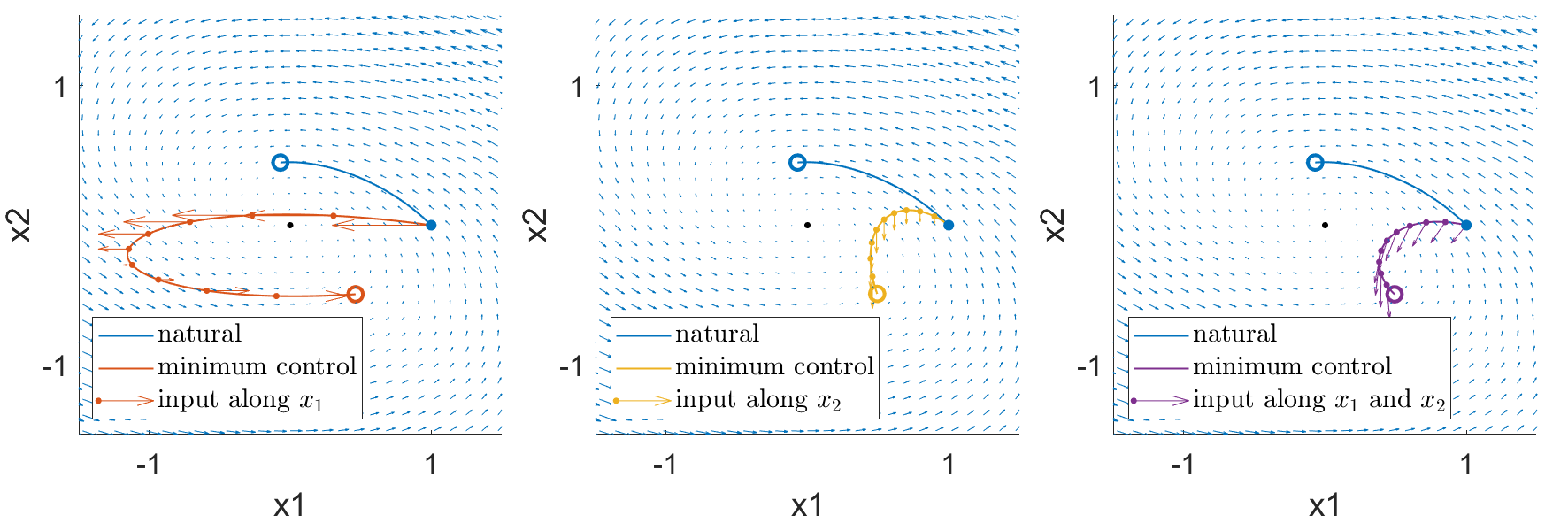
We observe that the state takes a rather roundabout trajectory to reach the target state, because the only way for the system state \(x_2\) to move downward is to push the state \(x_1\) to a regime where the natural dynamics allow \(x_2\) to decrease. Now, if we define a different control system where we can only influence the dynamics along the \(x_2\) state such that

\[\begin{split}\underbrace{\begin{bmatrix} \dot{x}_1\\ \dot{x}_2\end{bmatrix}}_{\dot{\mathbf{x}}} = \underbrace{\begin{bmatrix} -1 & -2\\ 1 & 0\end{bmatrix}}_{A} \underbrace{\begin{bmatrix} x_1\\ x_2\end{bmatrix}}_{\mathbf{x}} + \underbrace{\begin{bmatrix} 0 \\ 1\end{bmatrix}}_{B} \underbrace{\begin{bmatrix} u_1 \end{bmatrix}}_{\mathbf{u}},\end{split}\]

then we get the trajectory in the center subplot. Notice that the dynamics don’t push the system straight downard, but rather follows the natura dynamics upwards for a while before moving downard. This is because it costs less energy (input) to fight the weaker natural upward dynamics near the center of the vector field, as opposed to fighting the stronger natural upward dynamics near the right of the vector field.

Finally, if we are able to independently influence both of the system states,

\[\begin{split}\underbrace{\begin{bmatrix} \dot{x}_1\\ \dot{x}_2\end{bmatrix}}_{\dot{\mathbf{x}}} = \underbrace{\begin{bmatrix} -1 & -2\\ 1 & 0\end{bmatrix}}_{A} \underbrace{\begin{bmatrix} x_1\\ x_2\end{bmatrix}}_{\mathbf{x}} + \underbrace{\begin{bmatrix} 1 & 0\\ 0 & 1 \end{bmatrix}}_{B} \underbrace{\begin{bmatrix} u_1 \\ u_2 \end{bmatrix}}_{\mathbf{u}},\end{split}\]

then we get the controlled trajectory and inputs in the right subplot.