Inter-metric coupling across the principal gradient of functional connectivity

In this example, we illustrate how the cross-subject correlations between weighted degree and average controllability, as well as between weighted degree and modal controllability, vary as a function of the principal cortical gradient of functional connectivity. The data used here are structural connectomes taken from the Philadelphia Neurodevelopmental Cohort.

Here, our Python workspace contains subject-specific structural connectomes stored in A, a numpy.array with 200 nodes along dimensions 0 and 1 and 1068 subjects along dimension 3:

print(A.shape)

Out:
(200, 200, 1068)

We also have gradient, a numpy.array that designates where each of the 200 regions in our parcellation are situated along the cortical gradient:

print(gradient.shape)

Out:
(200,)

With these data, we’ll start by calculating weighted degree (strength), average controllability, and modal controllability for each subject:

# import
from tqdm import tqdm
from nctpy.utils import matrix_normalization
from nctpy.metrics import ave_control, modal_control

n_nodes = A.shape[0] # number of nodes (200)
n_subs = A.shape[2] # number of subjects (1068)

# strength function
def node_strength(A):
    str = np.sum(A, axis=0)

    return str

# containers
s = np.zeros((n_subs, n_nodes))
ac = np.zeros((n_subs, n_nodes))
mc = np.zeros((n_subs, n_nodes))

# define time system
system = 'discrete'

for i in tqdm(np.arange(n_subs)):
    a = A[:, :, i]  # get subject i's A matrix
    s[i, :] = node_strength(a)  # get strength

    a_norm = matrix_normalization(a, system=system)  # normalize subject's A matrix
    ac[i, :] = ave_control(a_norm, system=system)  # get average controllability
    mc[i, :] = modal_control(a_norm)  # get modal controllability

Next, for each region, we’ll calculate the cross-subject correlation between strength and average/modal controllability:

# compute cross subject correlations
corr_s_ac = np.zeros(n_nodes)
corr_s_mc = np.zeros(n_nodes)

for i in tqdm(np.arange(n_nodes)):
    corr_s_ac[i] = sp.stats.spearmanr(s[:, i], ac[:, i])[0]
    corr_s_mc[i] = sp.stats.spearmanr(s[:, i], mc[:, i])[0]

Plotting time! Below we illustrate how the above correlations vary over the cortical gradient spanning unimodal to transmodal cortex:

f, ax = plt.subplots(1, 2, figsize=(5, 2.5))
reg_plot(x=gradient, y=corr_s_ac,
         xlabel='regional gradient value', ylabel='corr(s,ac)',
         add_spearman=False, ax=ax[0], c=gradient)
reg_plot(x=gradient, y=corr_s_mc,
         xlabel='regional gradient value', ylabel='corr(s,mc)',
         add_spearman=False, ax=ax[1], c=gradient)
plt.show()

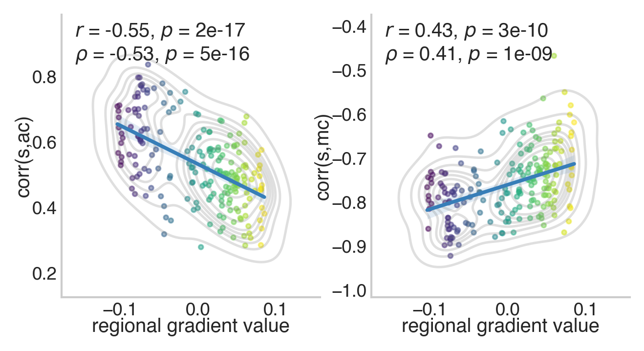
The above shows that the cross-subject correlations between strength and both average and modal controllability get weaker as regions traverse up the cortical gradient. The results for average controllability can also be seen in Figure 3a of Parkes et al. 2021.