Different approaches to computing minimum control energy
As discussed in Theory, there is more than one way to estimate the minimum control energy associated with a set of state transitions. Here, we compare our standard approach for calculating minimum control energy to an approach that leverages a shortcut based on vectorization. “why would I want to calculate control energy this way?” I hear you ask. The answer is simple: speed! As you’ll see below, the vectorization approximation provides highly convergent estimates of energy ~300 times faster than the standard approach.
The data used here are structural connectomes taken from the Philadelphia Neurodevelopmental Cohort.
Here, our Python workspace contains a single structural connectome stored in A, a numpy.array
with 200 nodes along dimensions 0 and 1.
print(A.shape)
Out:
(200, 200)
Before we calculate minimum control energy, we first need to define some brain states. Here, we’ll use
binary brain states, where each state comprises a set of brain regions that are designated as “on” (activity = 1) while
the rest of the brain is “off” (activity = 0). Just for illustrative purposes, we’ll define these brain states
arbitrarily by grouping the rows/columns of A into equally-sized non-overlapping subsets of regions.
# setup states
n_nodes = A.shape[0]
n_states = int(n_nodes/10)
state_size = int(n_nodes/n_states)

states = np.array([])
for i in np.arange(n_states):
    states = np.append(states, np.ones(state_size) * i)
states = states.astype(int)
The above code simply generates a vector of integers, stored in states, that designates which of 20 states each
brain region belongs to. Owing to the fact that n_nodes equals 200 here, each state comprises 10 nodes. Note, no nodes
are assigned to multiple states.
print(states)
Out:
[ 0  0  0  0  0  0  0  0  0  0  1  1  1  1  1  1  1  1  1  1  2  2  2  2
  2  2  2  2  2  2  3  3  3  3  3  3  3  3  3  3  4  4  4  4  4  4  4  4
  4  4  5  5  5  5  5  5  5  5  5  5  6  6  6  6  6  6  6  6  6  6  7  7
  7  7  7  7  7  7  7  7  8  8  8  8  8  8  8  8  8  8  9  9  9  9  9  9
  9  9  9  9 10 10 10 10 10 10 10 10 10 10 11 11 11 11 11 11 11 11 11 11
 12 12 12 12 12 12 12 12 12 12 13 13 13 13 13 13 13 13 13 13 14 14 14 14
 14 14 14 14 14 14 15 15 15 15 15 15 15 15 15 15 16 16 16 16 16 16 16 16
 16 16 17 17 17 17 17 17 17 17 17 17 18 18 18 18 18 18 18 18 18 18 19 19
 19 19 19 19 19 19 19 19]
So the first 10 nodes of A belong to state 0, the next 10 to state 1, and so on and so forth. Using these states,
we’ll first compute the minimum control energy required to transition between all possible pairs using our standard
function, nctpy.energies.get_control_inputs().
from nctpy.utils import matrix_normalization
from nctpy.energies import get_control_inputs, integrate_u

# settings
# time horizon
T = 1
# set all nodes as control nodes
B = np.eye(n_nodes)
# normalize A matrix for a continuous-time system
system = 'continuous'
A_norm = matrix_normalization(A, system=system)

import time
from tqdm import tqdm
start_time = time.time()  # start timer

# settings for minimum control energy
S = np.zeros((n_nodes, n_nodes))  # x is not constrained
xr = 'zero'  # x and u constrained toward zero activity

e = np.zeros((n_states, n_states))
for i in tqdm(np.arange(n_states)):
    x0 = states == i  # get ith initial state
    for j in np.arange(n_states):
        xf = states == j  # get jth target state
        x, u, n_err = get_control_inputs(A_norm=A_norm, T=T, B=B, x0=x0, xf=xf, system=system, xr=xr, S=S,
                                         expm_version='eig')  # get control inputs using minimum control
        e[i, j, :] = np.sum(integrate_u(u))

e = e / 1000  # divide e by 1000 to account for dt=0.001 in get_control_inputs

end_time = time.time()  # stop timer
elapsed_time = end_time - start_time
print('time elapsed in seconds: {:.2f}'.format(elapsed_time))  # print elapsed time
Out:
100%|██████████| 20/20 [01:35<00:00,  4.78s/it]
time elapsed in seconds: 95.68
The standard approach took ~95 seconds to calculate the control energy associated with completing 400 (20 x 20) state
transitions. Now we’ll compare that to our alternative approach, which is implemented in
nctpy.energies.minimum_energy_fast().
In order to use this variant of minimum control energy, we first
have to use our nctpy.utils.expand_states() function to convert states into a pair of boolean
matrices, x0_mat and xf_mat, that together encode all possible pairwise state transitions.
from nctpy.utils import expand_states
x0_mat, xf_mat = expand_states(states)
print(x0_mat.shape, xf_mat.shape)
Out:
(200, 400) (200, 400)
The rows of x0_mat and xf_mat correspond to the nodes of our system and the columns correspond to the states we
defined above. Critically, x0_mat and xf_mat are paired; if you take the same column across both matrices
you will end up with the initial state (x0_mat[:, 0]) and the target state (xf_mat[:, 0]) that comprise
a specific state transition. Note, nctpy.utils.expand_states() only works for binary brain states. If you
have non-binary brain states you’ll have to create x0_mat and xf_mat on your own. Equipped with these
state transition matrices, let’s compute energy again!
from nctpy.energies import minimum_energy_fast

start_time = time.time()  # start timer

e_fast = minimum_energy_fast(A_norm=A_norm, T=T, B=B, x0=x0_mat, xf=xf_mat)
e_fast = e_fast.transpose().reshape(n_states, n_states, n_nodes)
e_fast = np.sum(e_fast, axis=2)  # sum over nodes

end_time = time.time()  # stop timer
elapsed_time = end_time - start_time
print('time elapsed in seconds: {:.2f}'.format(elapsed_time))  # print elapsed time
Out:
time elapsed in seconds: 0.29
This time we managed to compute all of our transition energies in less than half a second! So our vectorization approach is fast, but is it equivalent?
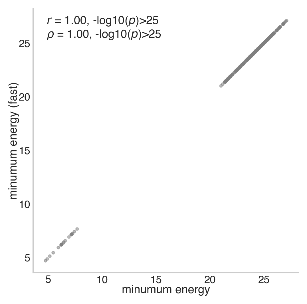
print(np.max(e - e_fast))
Out:
2.7267077484793845e-11
The largest difference between energies is tiny! Great, they’re pretty much the same. Let’s also visualize the energies using a correlation plot for good measure.
import matplotlib.pyplot as plt
from nctpy.plotting import set_plotting_params, reg_plot
set_plotting_params()

# plot
f, ax = plt.subplots(1, 1, figsize=(4, 4))

# correlation between whole-brain energy across state transitions
reg_plot(x=e.flatten(), y=e_fast.flatten(), xlabel='minumum energy', ylabel='minumum energy (fast)',
         ax=ax, add_spearman=True, kdeplot=False, regplot=False)
plt.show()
Note, there are several caveats to consider when using the above approach. First,
nctpy.energies.minimum_energy_fast() only works for continuous time systems. Second, the function does not
output the control inputs (u), state trajectory (x), or the numerical errors (n_err) provided by
nctpy.energies.get_control_inputs(). That is, you will only get node-level energy. Finally, as mentioned above,
nctpy.utils.expand_states() only works for binary brain states. This is trivial however; if you have non-binary
brain states you’ll just have to create x0_mat and xf_mat on your own.