Replication from White Matter Network Architecture Guides Direct Electrical Stimulation through Optimal State Transitions

Direct electrical brain stimulation is a useful treatment for some neurological disorders (most famously, Parkinson’s). However, we still don’t really have a good way of predicting how stimulation at a single region will influence the rest of the brain. Here, we hypothesize that input from stimulation will spread linearly along white matter tracts to impact brain activity at distant regions. We use a dataset of combined iEEG, DWI, and stimulation data to simulate stimulation based on this hypothesis.

In this example, we’re specifically going to ask if, given this model, it takes more stimulation energy to travel to more cognitively distant states. We’re going to define cognitive distance with the output from a classifier that guesses memory performance from brain states.

Data consist of one DWI structural adjacency matrix per dataset, and a variable number of stimulation trials. Each stimulation trial includes the brain state before and after stimulation.

The data used here are taken from the Restoring Active Memory Project.

Let’s take a look at the data:

import scipy.io as sio
workdir = '/Users/stiso/Documents/Code/test_data/'
subj = ['R1067P.PS1_set1','R1051J.PS1_set1','R1051J.PS1_set2.1', 'R1030J.PS1_set1', 'R1124J_1.PS2_set2',
        'R1124J_1.PS2_set3','R1124J_1.PS2_set1', 'R1150J.PS2_set1','R1150J.PS2_set2','R1170J_1.PS2_1_set1',
        'R1170J_1.PS2_1_set2','R1067P.PS1_set1','R1068J.PS1_set2.1','R1089P.PS2_set1','R1062J.PS1_set1',
        'R1173J.PS2_1_set1','R1066P.PS1_set1'];
dat = sio.loadmat(f'{workdir}Trajectory_Data.{subj[0]}.mat')
dat.keys()

Out:
dict_keys(['__header__', '__version__', '__globals__', 'Electrode_ROI', 'Post_Freq_State', 'Post_Stim_Prob',
'Pre_Freq_State', 'Pre_Stim_Prob', 'Stim_Amp', 'Stim_Duration', 'Stim_Freq', 'Stim_Loc_Idx', 'Struct_Adj'])

Here, the first important variable is Struct_Adj, which is our structural adjacency matrix (\(\mathbf{A}\)). Second is Pre_Freq_State, which is the band limited power in 8 frequencies, in all iEEG contacts, for each stimulation trial. This is our estimate of an initial brain state (\(x0\)). Because we have different frequency bands, we’re basically going to average across all of them to get one energy estimate (an alternative to this would be to vectorize all the frequency bands into one). The next important variable is Pre_Stim_Prob, which is the cognitive state at the start of every trial. High values indicate that someone is in a good cognitive state, or highly likely to encode a memory. The last useful variables are Stim_Loc_Idx, which tells us which contacts were used to stimulate on each trial, and Electrode_ROI, which helps us map between the iEEG contacts and the structural adjacency atlas.

If we’re gong to use optimal control, we’re missing a target state. We’re going use a good memory state as the target state. This is defined as an average of the 5% of states with the best classifier predictions for memory performance.

prefix = subj[0].split('_set')[0]
target = sio.loadmat(f'{workdir}targets/{prefix}.mat')
target.keys()

Out:
dict_keys(['__header__', '__version__', '__globals__', 'ROI_target'])

Now that we know what our data are, we can set the parameters for our optimal control model. These specific parameters were chosen to minimize the error of the optimal control calculation.

# balance between minimizing energy or minimizing distance from target state
rho = .2
# time to go from initial to target state
T = .7
# the number of time points the code spits out: T * 1000 + 1
nTime = 701
gamma = 4
# to try and simulate stimuluation, we're gonna weight the B matrix
B_mu = .0005
B_sigma = .00005

You’ll notice that there are a few new parameters here too, B_mu and B_sigma. Using optimal control to model stimulation with iEEG data presents some unique problems that these parameters help address. The first challenge is that we want to have input concentrated at stimulation electrodes, but having a sparse \(B\) matrix leads to very high error. The second challenge is that we dont have iEEG contacts in every region of the brain, so we have to guess at what those regions activity levels are. We therefore set the activity at all regions that dont have contacts to 1 (see the supplementary materials of Stiso et al. for evidence that the exact number doesn’t matter), but we also don’t want to waste a bunch of energy keeping these state values at 1 when we don’t really care about them. To address both these problems, we set the diagonal entries in \(B\) without corresponding electrodes to very small values drawn from a normal distribution defined by B_mu and B_sigma. This way, our \(B\) matrix is less sparse, our model will yield lower error, and states that we dont have recordings for will be able to regulate themselves.

Now we’re ready to get the optimal input required to go from any given starting state, to a good memory state. We expect that it is going to take more energy to go from bad to good states than good to good states.

from nctpy.utils import matrix_normalization
from nctpy.energies import get_control_inputs, integrate_u
import numpy as np
import pandas as pd
np.random.seed(0)

# intiialize final data strcutre
energies = pd.DataFrame(columns=['energy', 'condition', 'subject', 'trial', 'error'])

for i, s in enumerate(subj):
    prefix = subj[0].split('_set')[0]
    # load in data
    dat = sio.loadmat(f'{workdir}Trajectory_Data.{s}.mat')
    target = sio.loadmat(f'{workdir}targets/{prefix}.mat')

    # subject specific constants
    # number of stim trials for this set
    nTrial = np.size(dat['Post_Freq_State'], 0)
    # number of nodes/regions in the atlas we are using - one of the complications of this project is that we
    # dont have iEEG/state data for every regions of the atlas
    nROI = np.size(dat['Post_Freq_State'], 1)
    # number of bands
    nFreq = np.size(dat['Post_Freq_State'], 2)
    # these are the regions with contacts
    elec_idx = np.sum(dat['Post_Freq_State'][:, :, 0], 0) != 0
    ROI_idx = [not x for x in elec_idx]
    # number of contacts
    nElec = sum(elec_idx)
    # stim contacts
    stim_idx = [x[0][0] for x in dat['Stim_Loc_Idx']]

    # which regions we want to constrain the state of
    S = np.eye(nROI)

    # scale A matrix (continuous)
    # this variable will be the same for both datasets
    A = dat['Struct_Adj']
    A = matrix_normalization(A, c=gamma, system='continuous')

    # get optimal input and trajectory for each trial
    # each participant has a "good memory state", as determined by a linear classifier trained on memory performance
    xf = target['ROI_target']
    # this will take a while
    for t in range(nTrial):
        # get stim contacts
        e = stim_idx[t]

        # set sparse B matrix - ultimate goal is to have the majority of input be at the stim elecs
        # first, we set small input everywhere
        B = np.eye(nROI) * np.random.normal(loc=B_mu, scale=B_sigma, size=(1, nROI))
        # then we add 0s to all the areas whos activity we know
        B[elec_idx, elec_idx] = 0
        # then, we add big numbers to the stim elecs
        for c in e:
            B[c, c] = 1

        # get states
        x0 = np.squeeze(dat['Pre_Freq_State'][t, :, :])

        # add 1s to regions without elecs
        x0[ROI_idx, :] = 1

        # concatenate across frequency bands
        u = np.zeros((nROI, nTime, nFreq))
        err = np.zeros((1, nFreq))
        for f in range(nFreq):
            _, curr_u, curr_err = get_control_inputs(A, T, B, x0[:, f], xf[:,f], 'continuous', rho, S)

            curr_u = curr_u.T
            err[:, f] = curr_err
            u[:, :, f] = curr_u

        # get summary of optimal input
        # we incorporated the B matrix into our input summary because of the weighting
        # we use the term energy to be consistent with other literature, but in some sense this is a different summary statistic
        u = sum(np.linalg.norm(u.T*np.diag(B), axis=(0, 2)))/nTime

        # average over frequencies
        err = np.mean(err)

        # add to data frame (averaged over freqs)
        curr = pd.DataFrame({'energy':[np.mean(u)],
                            'initial_mem_state': dat['Pre_Stim_Prob'][0][t],
                            'subject':[s],
                            'trial':[t],
                            'error':[err]})
        energies = pd.concat([energies, curr], sort=False)

energies['log_eng'] = np.log(energies['energy'])
energies['log_err'] = np.log(energies['error'])

After a long time this will finish. Let’s first demonstrate that we have small error, since we went through a lot of trouble to make sure that was the case.

import seaborn as sns
import matplotlib.pyplot as plt
from nctpy.plotting import set_plotting_params
set_plotting_params()

fig, ax = plt.subplots(1, 2, figsize=(6, 3))
sns.histplot(energies, x='log_costate_err', hue='subject', stat='probability',
             ax=ax[0], palette='Blues_r', legend=False)
sns.histplot(energies, x='recon_error', hue='subject', stat='probability',
             ax=ax[1], palette='Blues_r', legend=False)
plt.tight_layout()
plt.show()

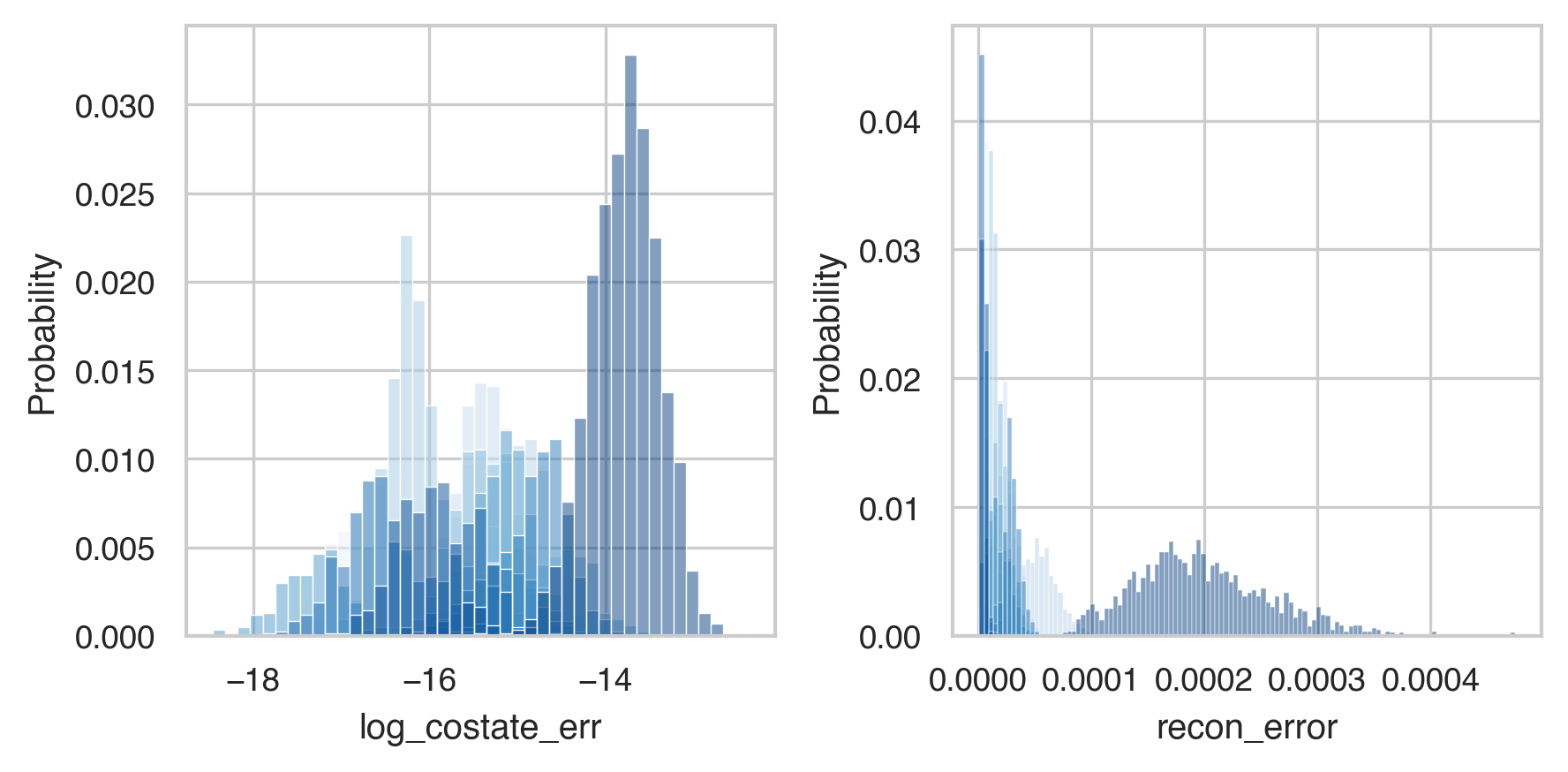
All the different datasets are in different shades of blue. And we can see here that everyone has low error values. Now lets check our actual hypothesis.

sns.lmplot(data=energies, y='log_eng', x='initial_mem_state', hue='subject', palette='Blues_r',
          height=3, aspect=2, legend=False)
plt.legend(bbox_to_anchor=(1.05, 1), loc=2, borderaxespad=0.)
plt.show()

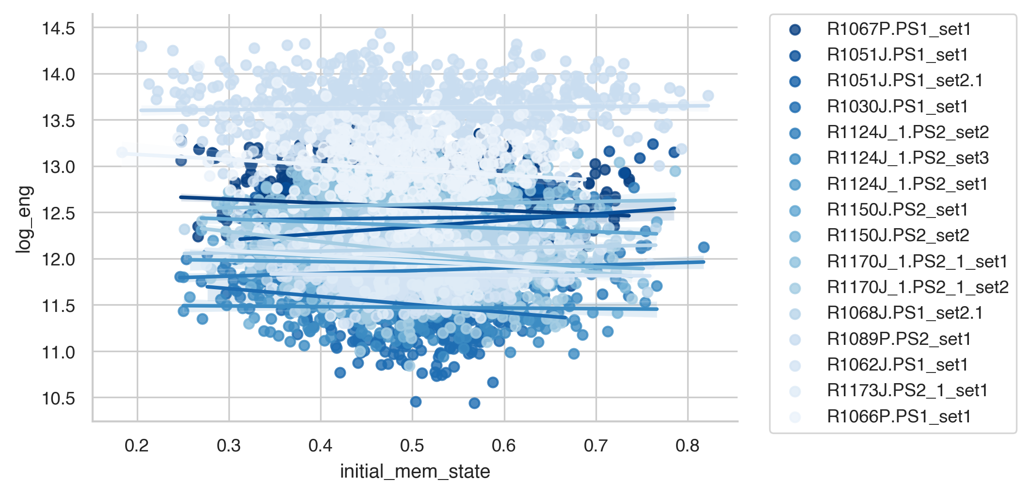
This plot looks a little different from the one in the paper because we don’t normalize the output. But as we can see, for most participants, transitions to good memory states require more energy when starting from a poorer memory state. In the paper, we show that the initial memory state explains more variance than the Euclidean distance between states as well.